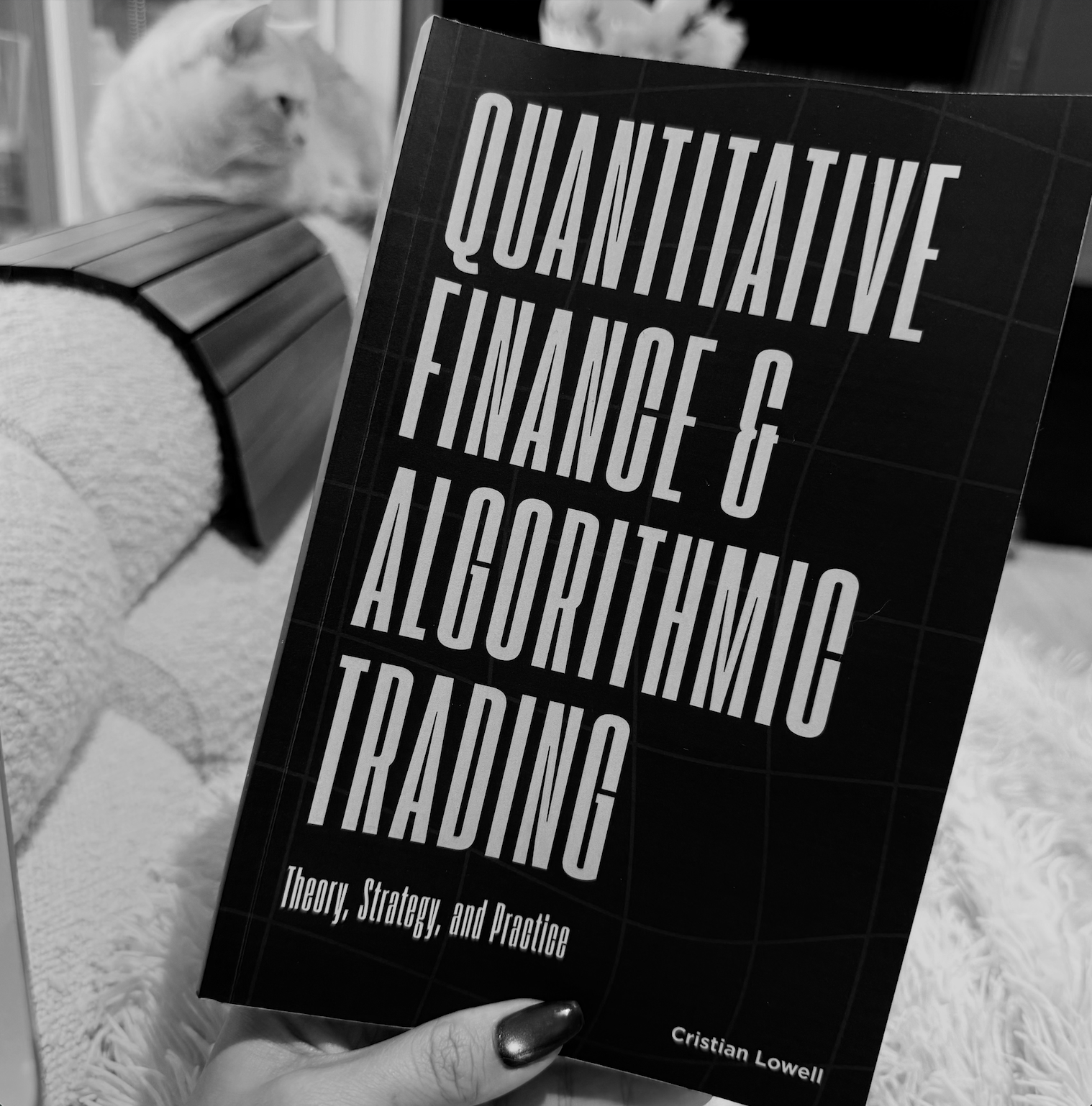
Quantitative Finance and Algorithmic Trading by Cristian Lowell

Really we’ve heard numerous times people use these two terms interchangeably.

Quantitative Finance and algorithmic trading.

Yet, they are not.

Some of the cleverest minds in finance never place a trade. Some of its busiest trading bots run on little more than baby arithmetic.

A quant researcher may spend an entire career pricing structured products or modelling the risks on a bank's balance-sheet without ever sending an order to market. Conversely, a rule as rudimentary as buying when the 50-day moving average crosses above the 200-day qualifies as algorithmic trading. Yet the two labels are routinely conflated, not least because the same people often switch between them within a single afternoon. That muddle is the starting point of Quantitative Finance and Algorithmic Trading: Theory, Strategy, and Practice by Cristian Lowell.

The author Lowell illustrated that the two disciplines overlap heavily, though neither is a subset of the other, and that a viable strategy requires both. Quantitative finance identifies a genuine, well-evidenced source of edge; algorithmic trading harvests it systematically, and swiftly enough to do so before the opportunity evaporates. Neglect either and the enterprise founders: insight without disciplined execution bleeds money through slippage and delay, while execution without insight is just automating a coin flip. Most of the book analyzed that overlap, where a statistical-arbitrage strategy is both devised and executed by machine.

This is not a book of trading secrets or flattering backtests. Lowell computes every result, checks it twice and reports what the numbers show, even when they disappoint. Each model is held up against an independent method: Monte Carlo simulation against the closed-form Black–Scholes price, out-of-sample performance against in-sample fit, a formal cointegration test against a chart that merely looks convincing. Three simulated datasets, each generated with a fixed random seed, run through the technical chapters, and a fictional fund, Ashgrove Quantitative Partners, carries the methods into practice. Closing case studies on the collapse of Long-Term Capital Management in 1998, the storied record of Renaissance Technologies and the "flash crash" of May 2010 then put the ideas to the test of real history.

So why are the two terms often confused?

Quantitative finance is the broad discipline of applying mathematics, statistics and computation to financial problems: pricing derivatives, measuring risk, building portfolios. Much of it never places a trade. A bank's risk quant estimating expected shortfall is doing quantitative finance.

Algorithmic trading is narrower: computer programs that submit and manage orders by predefined rules on timing, price and size. It needs no forecasting model. A broker's algorithm that slices a large order to match the volume-weighted average price has no view on the market at all:

VWAP = Σᵢ pᵢ vᵢ / Σᵢ vᵢ

So why are they confused? First, they grew up together. Decimal pricing, completed in US markets in 2001, and electronic order books made it possible both to model markets with fine-grained data and to trade them by machine, and the firms that did one usually did the other. Second, they share a toolkit: Python, historical data and backtests look the same whether they serve a pricing model or an execution engine. Third, the language blurred. "Quant" became shorthand for anyone who codes at a trading firm, retail platforms sell rule-based bots as "quant trading", and coverage of high-frequency trading and the 2010 Flash Crash lumped models and machines together.

The two fields meet in quantitative trading, where a model decides what to trade and an algorithm decides how. Treating them as one hides that a strategy can fail at either stage. A flawless algorithm will execute a worthless signal perfectly, and Lowell's momentum result is a failure of this first kind. A sound strategy can also be undone by its machinery, as Knight Capital learned in 2012. The rest of the book, and this review, follows that split: first the mathematics both halves rest on, then the research that decides what to trade, then the execution that decides how.

What to trade: quantitative finance

The next five sections cover quantitative finance: the mathematics and research that decide what a strategy should trade.

Every model that follows, from option pricing to position sizing, needs an assumption about how prices move. The standard starting point is geometric Brownian motion, in which a price drifts at rate μ and is shaken by volatility σ through a Wiener process W:

dSₜ = μ Sₜ dt + σ Sₜ dWₜ

To work with this equation, you need a calculus for random paths. Because W is nowhere differentiable, ordinary calculus fails; Itô's lemma adds a second-order correction, and applied to the log price it gives:

d ln Sₜ = (μ − ½σ²) dt + σ dWₜ

The −½σ² term, known as volatility drag, is why average arithmetic returns overstate compounded growth, and it returns at the end of the book when bets are sized. Real returns also show excess kurtosis, with far more extreme moves than a normal distribution allows, and every later test statistic inherits that problem.

With a model of single prices in place, the first question on the "what to trade" side is what to hold. Harry Markowitz's 1952 answer is to choose weights that minimise variance for a target return m:

min over w: ½ wᵀΣw, subject to wᵀμ = m and wᵀ𝟏 = 1

Adding a risk-free asset at rate r_f reduces the whole efficient frontier to one best mix of risky assets, the tangency portfolio:

w* = Σ⁻¹(μ − r_f 𝟏) / 𝟏ᵀΣ⁻¹(μ − r_f 𝟏)

This is where Lowell's insistence on testing matters. The formula needs Σ⁻¹, and inverting a noisy estimate magnifies its errors, which led Richard Michaud in 1989 to describe optimisers as "estimation-error maximisers". The standard fix is Ledoit–Wolf shrinkage, which pulls the sample covariance S towards a structured target F:

Σ̂ = δF + (1 − δ)S

Choosing a portfolio also means measuring how badly it can lose. Value at Risk gives a loss threshold but ignores what lies beyond it and is not subadditive. Expected Shortfall averages the tail itself, which is why Basel regulators adopted it for market risk:

ES(α) = 𝔼[L | L ≥ VaR(α)]

We use portfolios to decide what to hold; and we use derivative to ask what a contingent claim is worth. They are also the clearest test of the book's cross-checking method, because one price can be computed three independent ways. The derivation starts with a hedge: hold an option V and short Δ = ∂V/∂S shares, and Itô's lemma cancels the random terms. A riskless portfolio must earn the risk-free rate r, which gives the Black–Scholes equation of 1973:

∂V/∂t + ½σ²S² ∂²V/∂S² + rS ∂V/∂S − rV = 0

The drift μ disappears: an option's price does not depend on the stock's expected return. Solving the equation for a European call with strike K and expiry T gives the first of the three methods, a closed form:

C = S₀ N(d₁) − Ke⁻ʳᵀ N(d₂), where d₁,₂ = [ln(S₀/K) + (r ± ½σ²)T] / (σ√T)

The second method is risk-neutral Monte Carlo, which the Feynman–Kac theorem links to the same equation: C = e⁻ʳᵀ 𝔼[max(S(T) − K, 0)], with the expectation taken under the risk-neutral measure ℚ. The third is the Cox–Ross–Rubinstein binomial tree. If the three disagree, the code is wrong, which is exactly the kind of check Lowell builds into every chapter.

Pairs that drifts together

In August 2007, many quantitative long-short equity funds lost heavily within days while the broader market barely moved. Andrew Khandani and Andrew Lo traced it to crowded, similar positions being unwound at once.

That episode shows why a trading relationship has to be proven before money goes behind it. Statistical arbitrage bets that two related prices will converge, so Lowell first checks whether the relationship exists at all, using formal statistical tests. Under Engle and Granger's 1987 framework, the spread sₜ = yₜ − βxₜ must be stationary, which the augmented Dickey–Fuller test checks:

Δsₜ = α + γ sₜ₋₁ + Σᵢ₌₁ᵖ φᵢ Δsₜ₋ᵢ + εₜ

The null is γ = 0, a unit root. Because β is itself estimated, the usual t critical values do not apply, and Johansen's test is needed for more than two assets. Once a spread passes, the trader needs to know how fast it reverts, since that sets holding periods and stop-losses. The Ornstein–Uhlenbeck process models this, with half-life ln 2 / θ:

dXₜ = θ(μ − Xₜ) dt + σ dWₜ

Markets change over time, so two refinements keep the model up to date. A Kalman filter lets the hedge ratio β drift, and GARCH(1,1) lets the spread's volatility change, capturing the clustering in which turbulent days follow turbulent days:

σₜ² = ω + α εₜ₋₁² + β σₜ₋₁²

Machine Learning and the Noise Problem

Machine learning promises to find the signals simpler models miss, which makes it the easiest place to fool yourself. The bias–variance decomposition shows why that promise is hard to keep in markets:

𝔼[(y − f̂(x))²] = Bias² + Variance + σ²

In returns data the noise term σ² dominates, so extra flexibility mostly buys variance. Ordinary k-fold cross-validation leaks information across overlapping return windows; purged and embargoed cross-validation fixes this.

A second trap explains why so many published backtests look better than they are: test enough strategies and the best will look good by chance. David Bailey and Marcos López de Prado estimate the expected maximum Sharpe ratio among N worthless strategies, with γ the Euler–Mascheroni constant:

𝔼[max SR̂] ≈ √V[SR̂] · ( (1 − γ) Φ⁻¹(1 − 1/N) + γ Φ⁻¹(1 − 1/(Ne)) )

That value becomes the benchmark SR* in the probabilistic Sharpe ratio, which also corrects for track-record length T, skewness γ₃ and kurtosis γ₄. The result is the deflated Sharpe ratio:

PSR(SR*) = Φ( (SR̂ − SR*) √(T − 1) / √(1 − γ₃ SR̂ + ((γ₄ − 1)/4) SR̂²) )

Held to this standard, the momentum effect documented by Narasimhan Jegadeesh and Sheridan Titman in 1993 shrinks in Lowell's tests: most of its edge turns out to be noise.

How to trade: algorithmic trading

From here the review turns to algorithmic trading: how an order reaches the market, what it costs, and how a strategy runs as a live process.

The algorithmic half starts with a basic question: why does trading move prices at all? In Albert Kyle's 1985 model, an insider knows an asset's true value, noise traders submit random orders, and a market maker sets the price linearly in total order flow y. With prior variance Σ₀ and noise-trading volatility σᵤ:

Δp = λy, where λ = ½ √Σ₀ / σᵤ

Kyle's λ is the price of liquidity. In Glosten and Milgrom's model, the market maker sets the ask at 𝔼[v | buy] and the bid at 𝔼[v | sell], so the spread is the cost of adverse selection.

Once impact has a price, a large order becomes an optimisation problem: trade fast and pay impact, trade slowly and risk the price moving away. Robert Almgren and Neil Chriss's 2000 framework balances the two by minimising 𝔼[C] + λ Var[C]. With linear impact, the optimal holdings decay as:

xⱼ = X · sinh(κ(T − tⱼ)) / sinh(κT), where κ ≈ √(λσ² / η)

A risk-neutral trader spreads the order evenly; a risk-averse one front-loads it. Empirically, impact grows roughly with σ√(Q/V), the square-root law. A small edge per trade can vanish into these costs.

A strategy that passes every test still has to run, and this is where both halves of Lowell's argument meet. On 1 August 2012, Knight Capital lost about $440 million in roughly 45 minutes after a faulty software deployment sent a flood of unintended orders into the market. The book's seventh part moves a strategy from research to a running process, using Ashgrove Quantitative Partners as the setting.

Running a fund raises two final questions: how many bets to make, and how large each should be. For the first, Richard Grinold's fundamental law links a manager's information ratio to skill per bet (IC) and the number of independent bets a year (BR):

IR ≈ IC × √BR

An IC of 0.05 across 1,000 bets beats an IC of 0.2 across ten, provided the bets really are independent, which August 2007 showed they often are not. For the second question, the Kelly criterion gives the leverage that maximises long-run growth, and the −½σ² drag from Itô's lemma reappears:

f* = μ / σ², and g(f) = r + fμ − ½f²σ²

Because μ is estimated with error and overbetting costs more than underbetting, practitioners trade a fraction of full Kelly.

Lowell's answer to his opening question is that a strategy is two problems: a quantitative question of what to trade and an algorithmic question of how. Keeping them apart, and reporting honestly when either fails, is the book's real contribution. Through Lowell's lens, an optimiser becomes a problem of estimation error, a pairs trade a hypothesis to test, and a machine learning model a candidate that must beat noise.

This book has its limits ofcourse. It is meant to be introductory which leaves little room for each topic, and a full treatment of stochastic calculus or derivatives theory still needs the more texts. Because the results come from generated data, they show how each method behaves under known conditions, and readers will still need to test them on real markets.

Personally, I find it as a rewarding read for beginners heading into quantitative roles, self-taught traders who want to stress-test their backtests, and practitioners tired of books that promise more than the data supports.